Reanalyzing Public Datasets

To illustrate the use case of the Omics Playground, we reanalyzed different types of publics datasets, including microarray, bulk RNA-seq, single-cell RNA-seq and proteomic datasets to recapitulate the results.

Single-cell RNA-seq data

For single-cell RNA-seq data, we downloaded the melanoma data set GSE72056 of Tirosh et al.. Our platform recapitulates well the original findings of the paper. The t-SNE clustering (Figure 1) separates the different cell types. Figure 2 and Figure 3 show the volcano plot, MA plot and most differentially expressed genes between malignant and non-malignant cells. The CNV map (Figure 4) confirms the major chromosomal copy number variations found in the malignant cells. Figure 5 shows high enrichment of a immune checkpoint signature, particularly concentrated in the T cells. The biomarker heatmap (Figure 6) highlights the marker genes for each cell type. Each gene cluster is furthermore automatically annotated with the most correlated gene sets (Figure 7).

tSNE plot

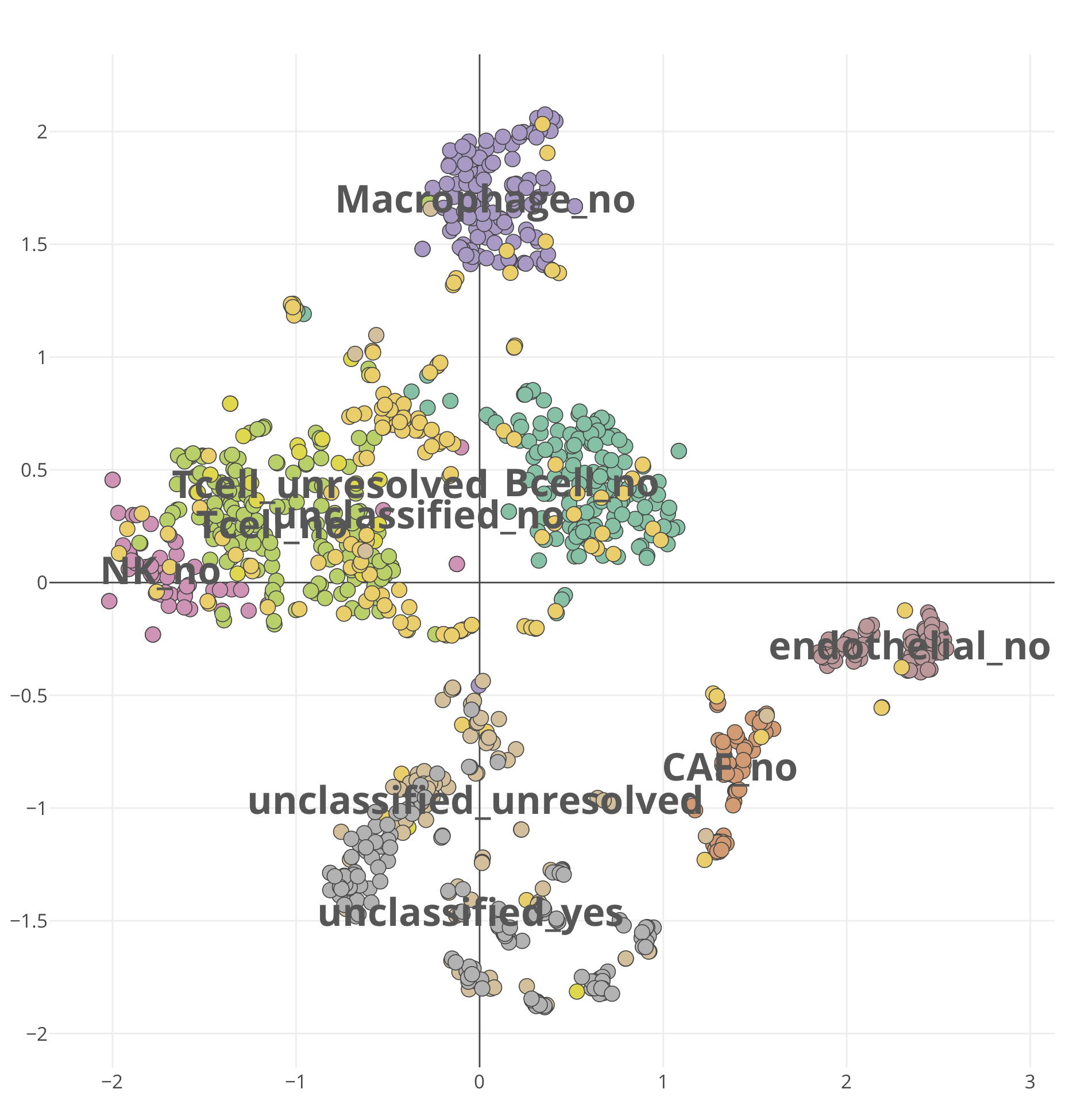
Figure 1. The t-SNE clustering with cell type annotation for the GSE72056-scmelanoma dataset. To reproduce the figure on the platform, select and load GSE72056-scmelanoma dataset, and go to the PCA/tSNE panel of the Clustering module. From the plot Settings, set the color: group, layout: tsne, and leave other settings as default.

Volcano and MA plot

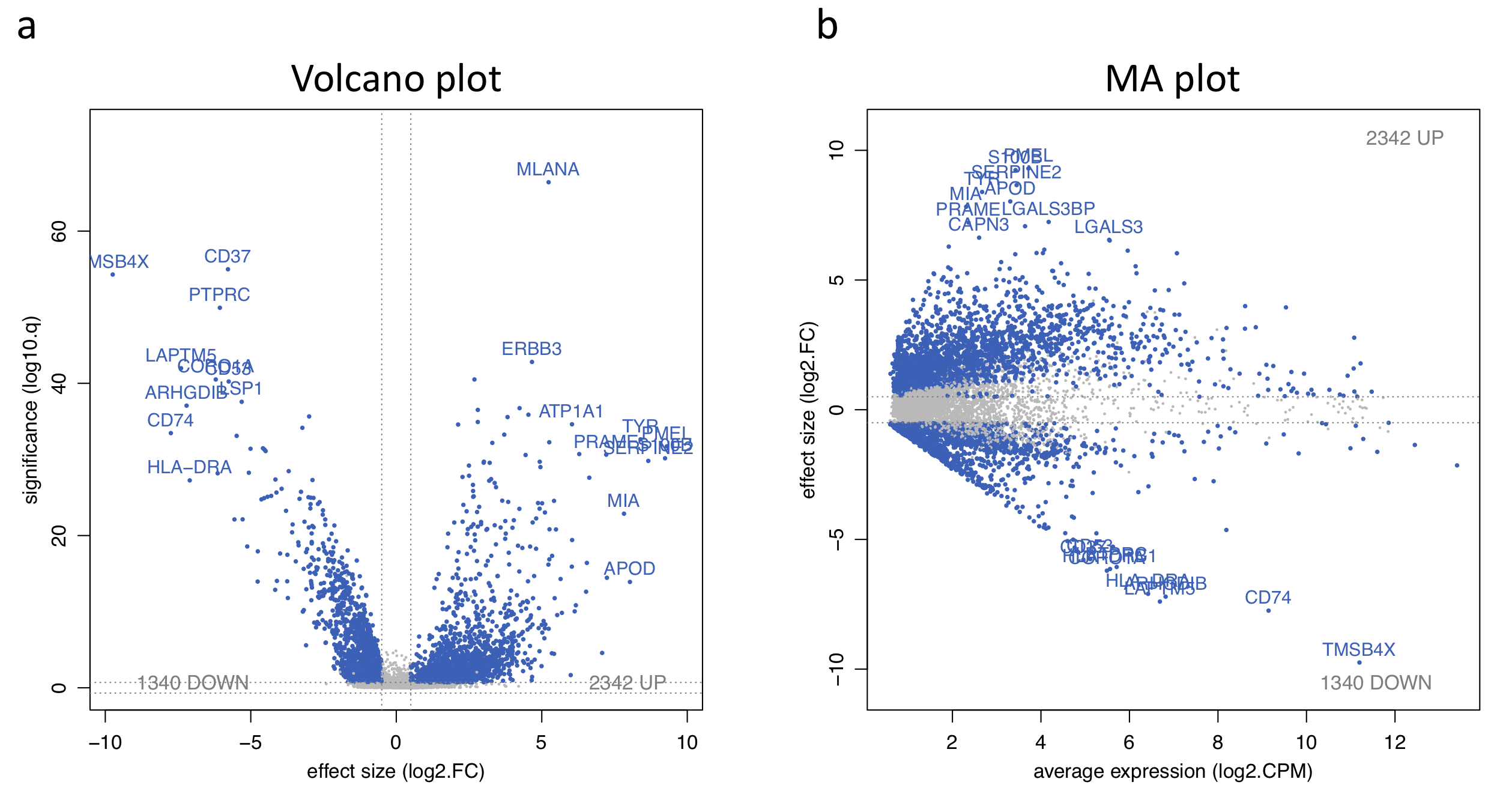
Figure 2. Volcano and MA plot for the malignant versus non-malignant contrast. To replicate the figure on the platform, go to the Plots panel of the Expression module. From the input slider, set the Contrast: yes_vs_no and Gene family: all.

Differentially expressed genes

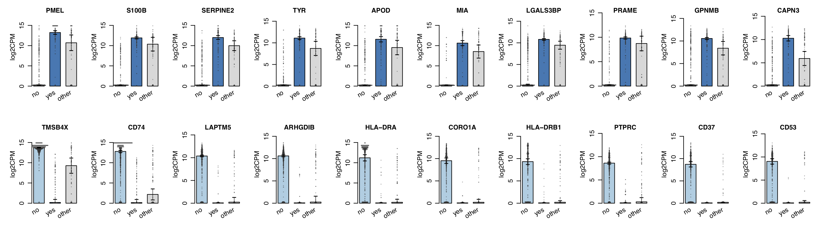
Figure 3. Barplot of corresponding differentially expressed genes. To obtain the figure on the platform, go to the Top genes panel of the Expression module. From the input slider, set the Contrast: yes_vs_no and Gene family: all.

Inferred copy number

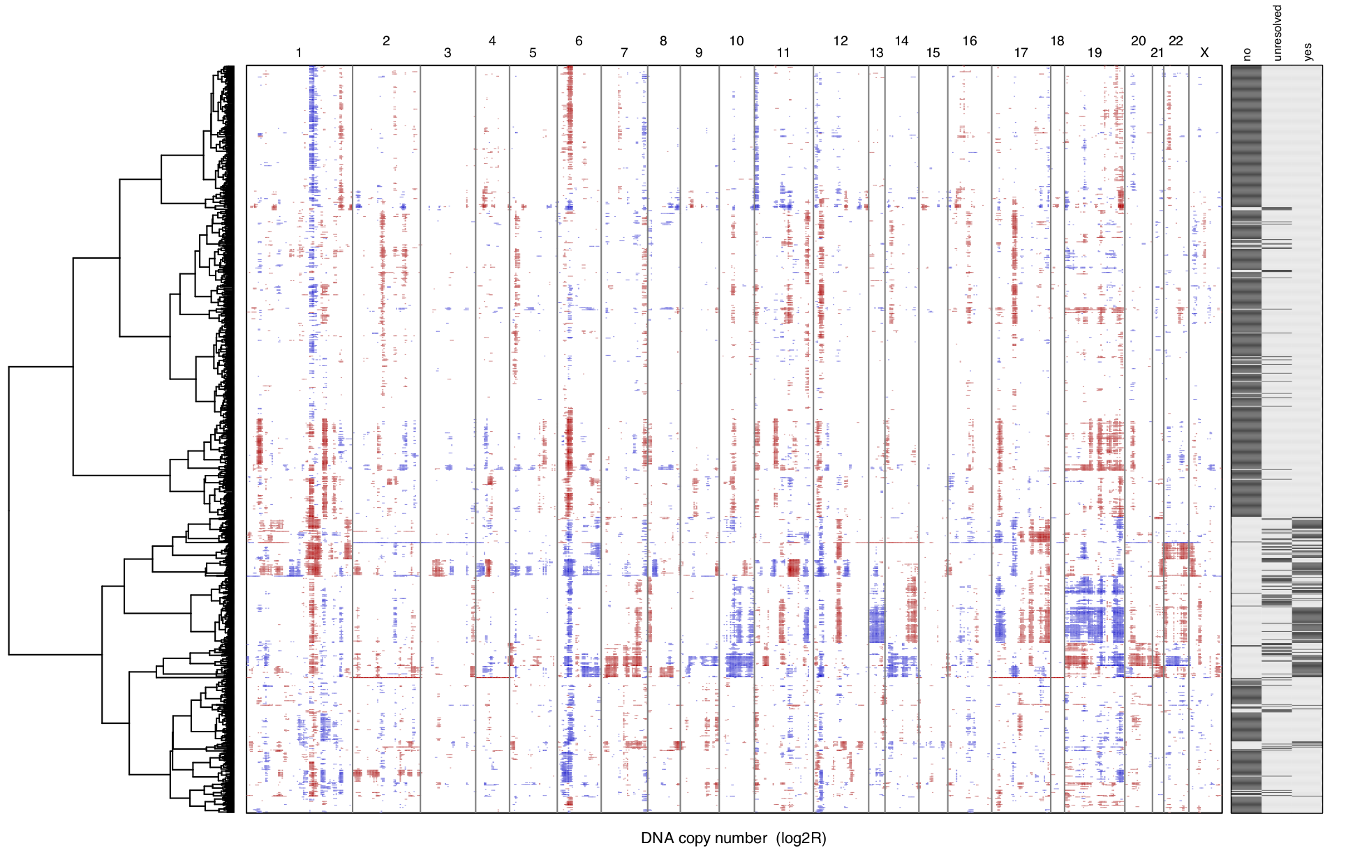
Figure 4. Inferred copy number for sample Cy80. To reproduce the figure on the platform, go to the CNV panel of the scProfiling module. From the plot Settings, set the Annotate with: malignant and Order samples by: clust.

Immune checkpoint signature

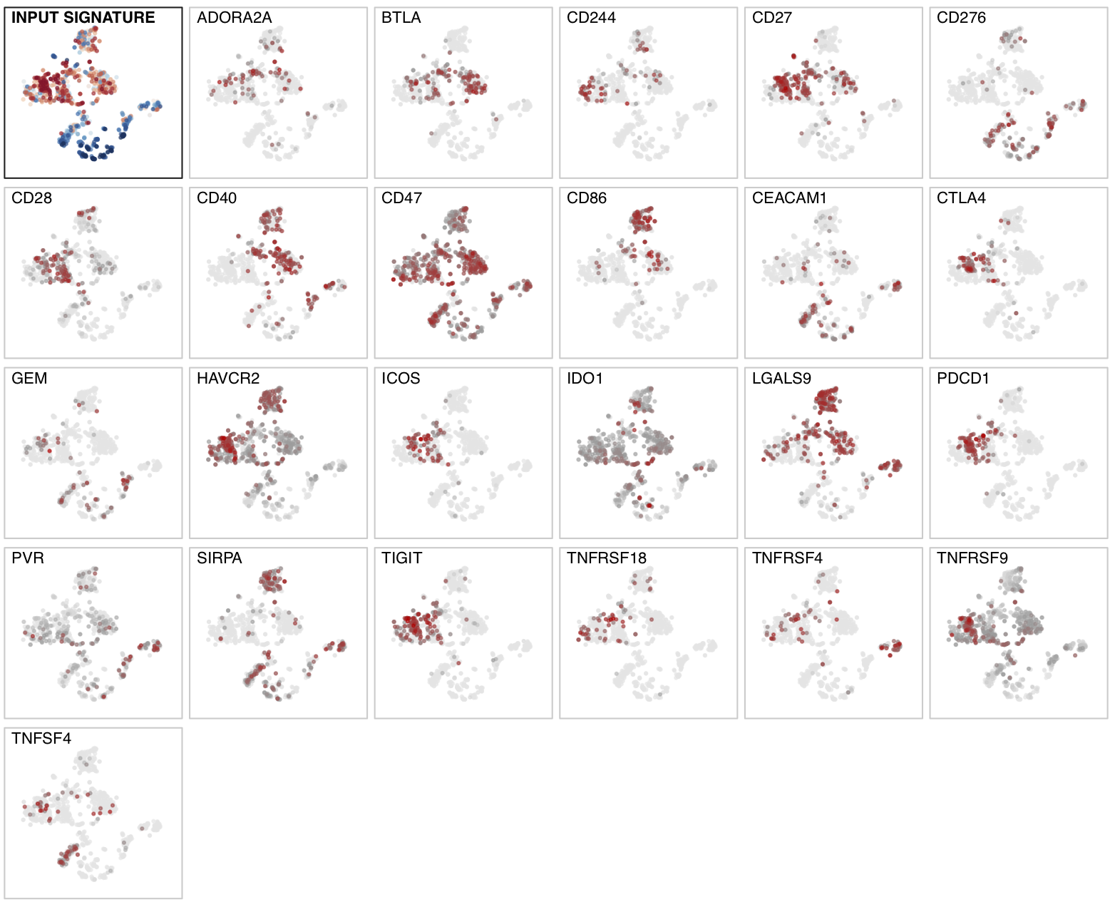
Figure 5. Enrichment distribution for an immune checkpoint signature showing high enrichment in T and B cells . To regenerate the figure on the platform, go to the Marker panel in the Signature module. From the input slider, select Contrast: custom and Signature: immune_chkpt as it is provided in the sample list.

Biomarker heatmap

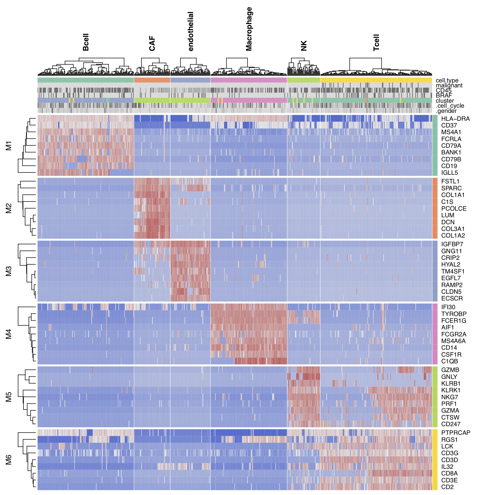
Figure 6. Biomarker heatmap for non-malignant cells. To reproduce the figure on the platform, go to the Heatmap panel in the Clustering module. From the input slider, set the Filter samples: cell.type={Bcell, CAF, endothelial, Macrophage, NK, Tcell}. In the plot Settings, set Plot type: ComplexHeatmap, split by: cell.type, and top mode: specific.

Annotate heatmap clusters

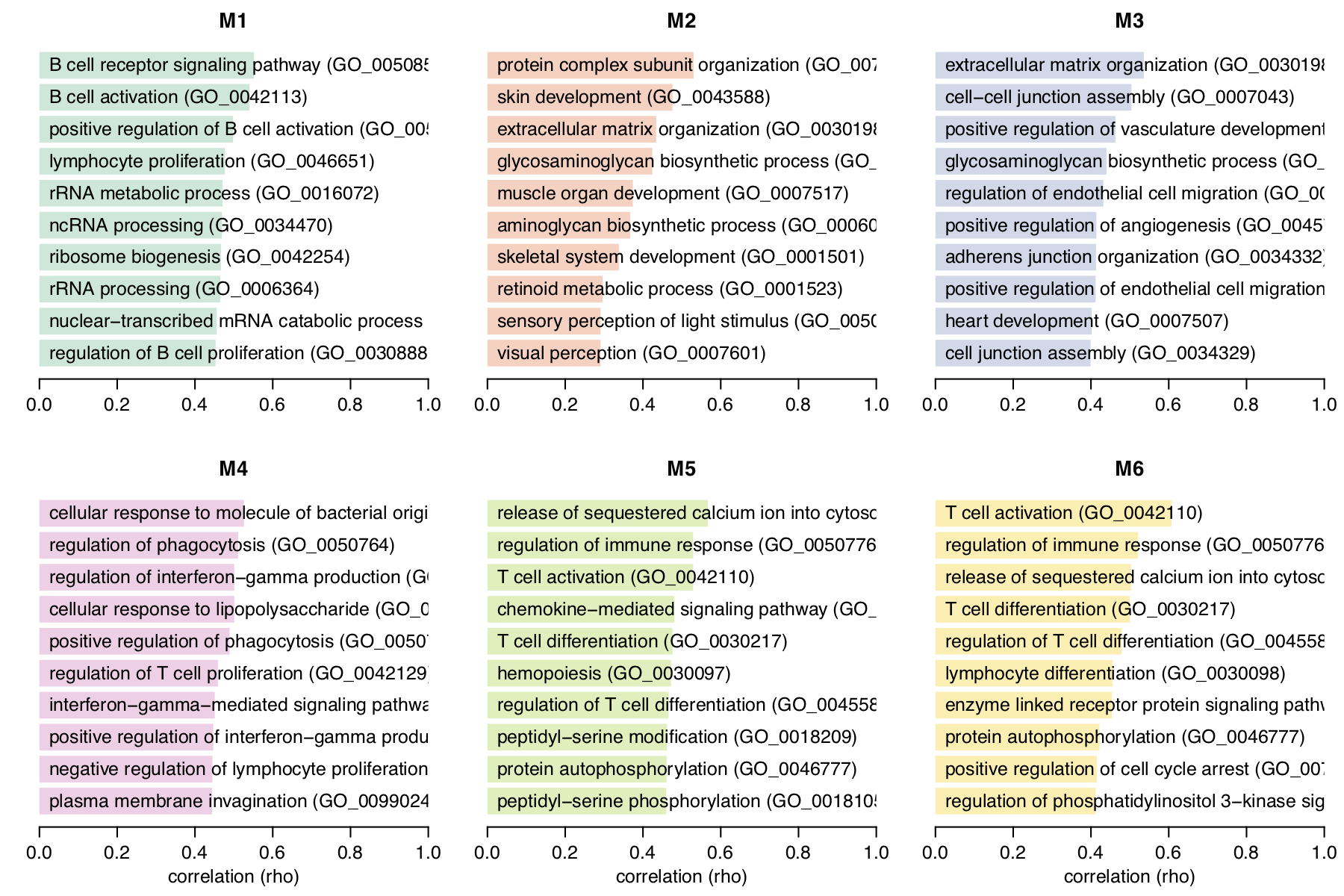
Figure 7. Enrichment annotation of corresponding heatmap clusters from the Figure 6. To reproduce the figure on the platform, generate the heatmap in Figure 6 first, then go to the Annotate clusters panel. From the plot Settings, set the Reference set: GOBP.

Bulk RNA-seq Data

To elucidate the mechanism of action of a new drug, or for the intention of drug repurposing, it is often useful to find other drugs that have similar or opposing signatures compared to some given fold change profile. This example is illustriated using the RNA-sequencing dataset GSE114716 from Goswami et al., which contains CD4 T cells following ipilimumab therapy. Figure 8 shows the top ranked drugs with most similar or most opposing signatures to ipilimumab, a novel monoclonal antibody targeting CTLA-4 used in tumour therapy to stimulate the immune system. The complete list contains several compounds that stimulate the immune system, such as alpha-tocopherol (Morel et al.), but also highlights compounds that are not commonly associated with the modulation of immune responses, such as strophanthidin, an intropic drug that has recently been shown to display pro-inflammatory activities (Karas et al.).

Drug enrichment profiles

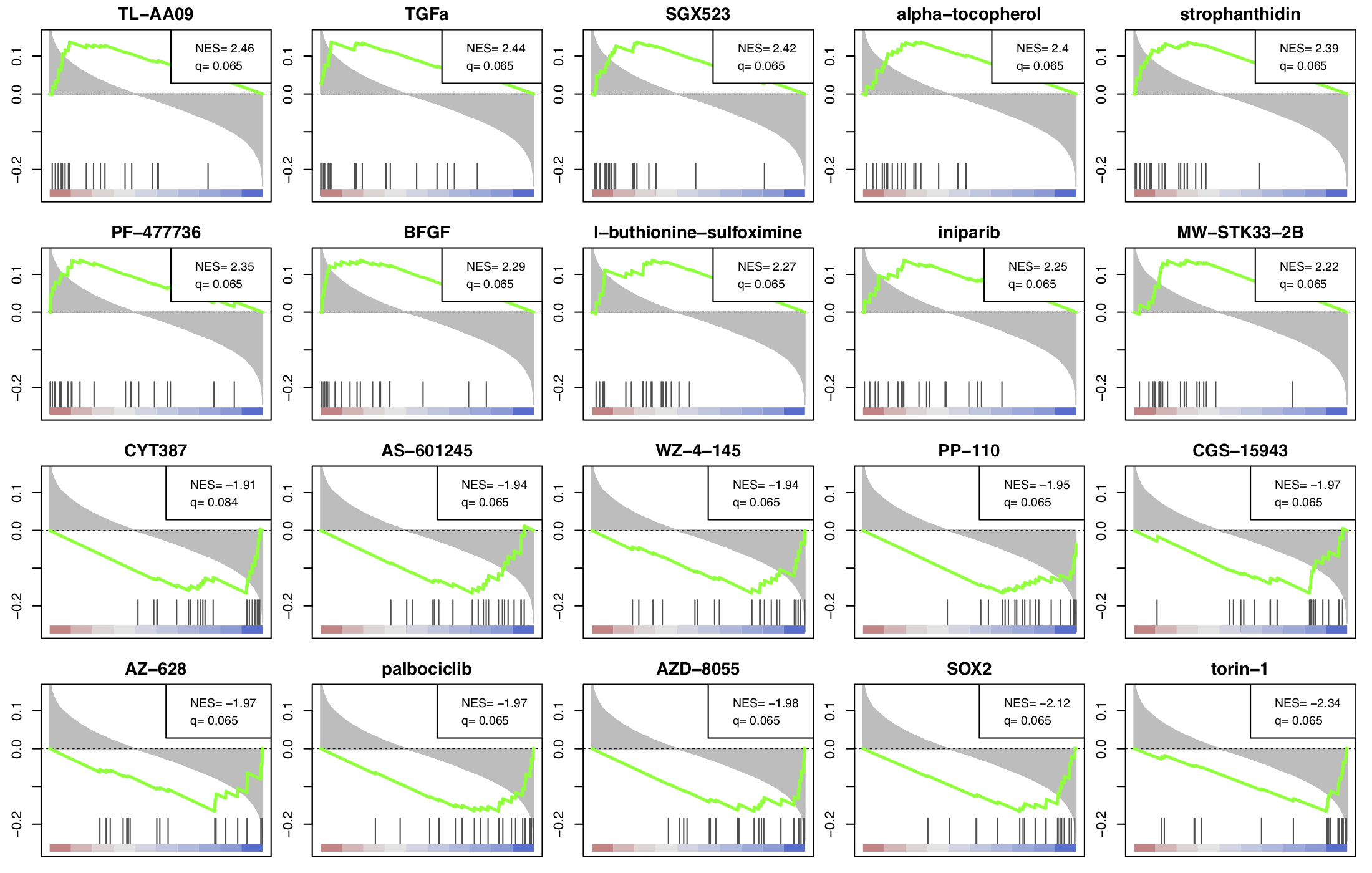
Figure 8. Drug enrichment profiles for most similar and opposing drugs compared to ipilimumab treatment. To reobtain the figure on the platform, select and load GSE114716-ipilimumab dataset, go to the Drug CMap panel under the Functional module, and set the Contrast: Ipi_vs_baseline from the plot Settings.

Microarray Data

In this section, we perform the heatmap clustering, biomarker selection and survival analysis using the GSE10846 from Lenz et al., which is the microarray gene expression dataset of diffuse large B-cell lymphoma (DLBCL) patients. Figure 9 shows a hierarchical cluster heatmap of microarray gene expression data. Figure 10 and Figure 11 show the variable importance plot and a survival tree on the overall survival of the DLBCL patients, respectively.

Hierarchical cluster heatmap

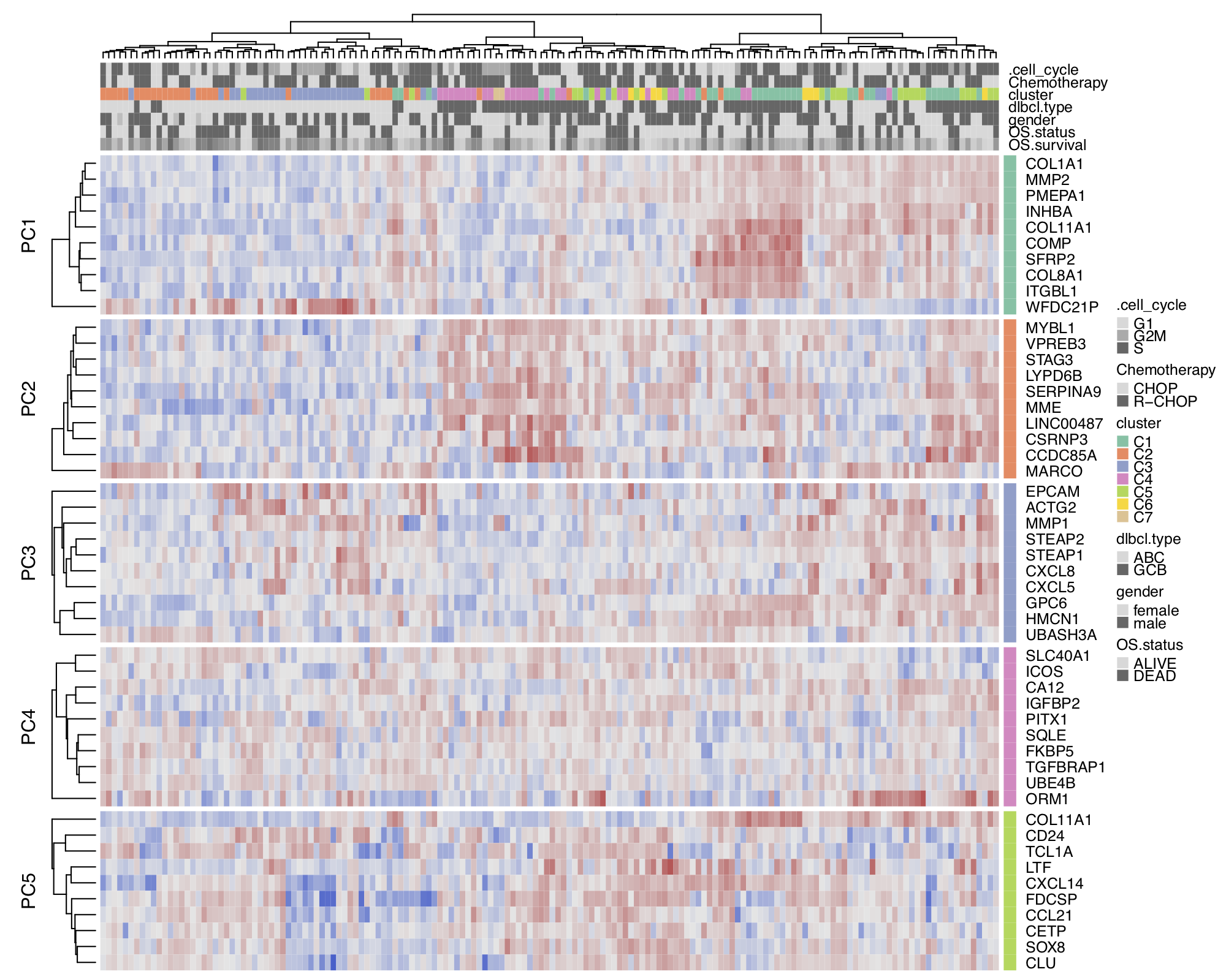
Figure 9. Hierarchical cluster heatmap for GSE10846-dlbcl dataset. To replicate the figure, select and load GSE10846-dlbcl dataset on the platform. Go to the Heatmap panel of the Clustering module, and set the Level: gene and Features: all from the input panel. In the plot Settings, set the split by: none and Top mode: pca.

Variable importance plot

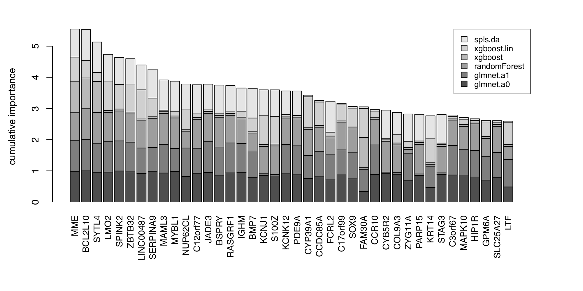
Figure 10. Variable importance plot. To replicate the figure, go to the Biomarker module, and set the Predicted target: dlbcl.type from the input panel.

Survival tree

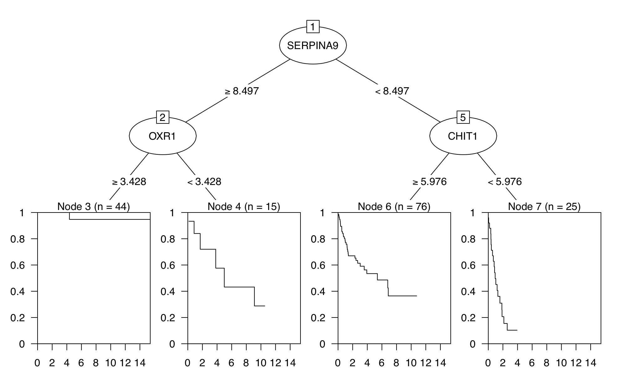
Figure 11. Survival tree analysis for GSE10846-dlbcl dataset. To redproduce similar figures, go to the Biomarker module, and set the Predicted target: OS.survival from the input panel. Note that the survival tree is stochastically built up with some of the top features shown in Figure 10; Therefore, users can get a slightly different survival tree every time.

Proteomic Data

With larger data sets, often the number of contrasts increases and complicates the overall analysis. For example, the proteomics data set of Rieckmann et al. 2017 comprises 26 populations of seven major immune cell types, measured during resting and activated states. There are more than 300 possible comparisons to make. To gain a better overview, gene set activation matrix (Figure 12) help visualize the similarities between multiple contrasts on a functional level. Alternatively, similarities can be visualized as a connectivity graph (Figure 13). For the same data set, Figure 14 shows a computed partition tree that classifies the major cell types.

Another example dataset is from Geiger et al., where the proteome profiles of activated vs resting human naive T cells at different times were compared. Figure 15 shows the volcano plots corresponding to eight different statistical tests comparing time-dependent activation of T cells at 48h vs. 12h. We see that both standard t-test and the Welch t-test show much less power to detect significant genes compared to the other methods. The result from edgeR-QLF is close to those of the two limma based methods, while edgeR-LRT is very similar to the results of DESeq2-Wald.

Activation matrix

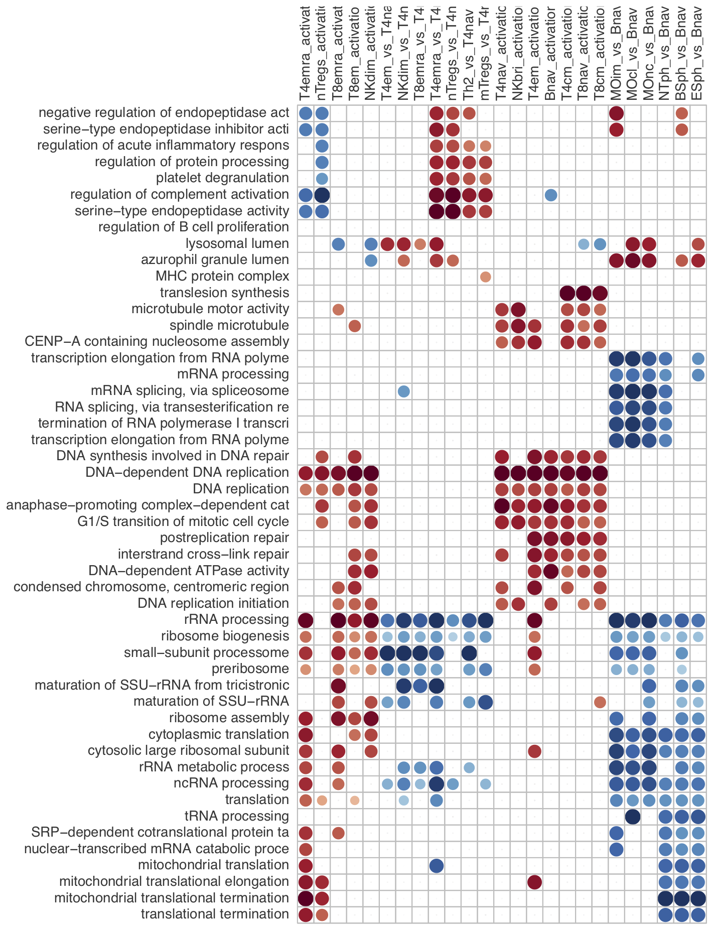
Figure 12. Gene Ontology activation matrix. To replicate the figure, select and load the rieckmann2017-immprot dataset, and go to the GO graph panel of the Functional module with default settings.

Contrast heatmap

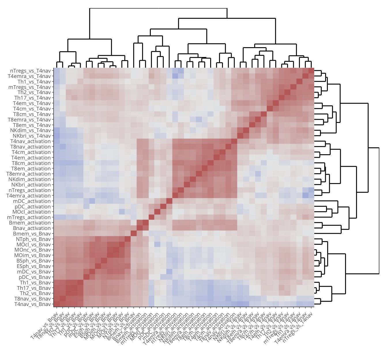
Figure 13. Contrast heatmap for the rieckmann2017-immprot dataset. To generate the figure on the platform, go to the Contrast heatmap panel of the Intersection module with default settings.

Classification tree

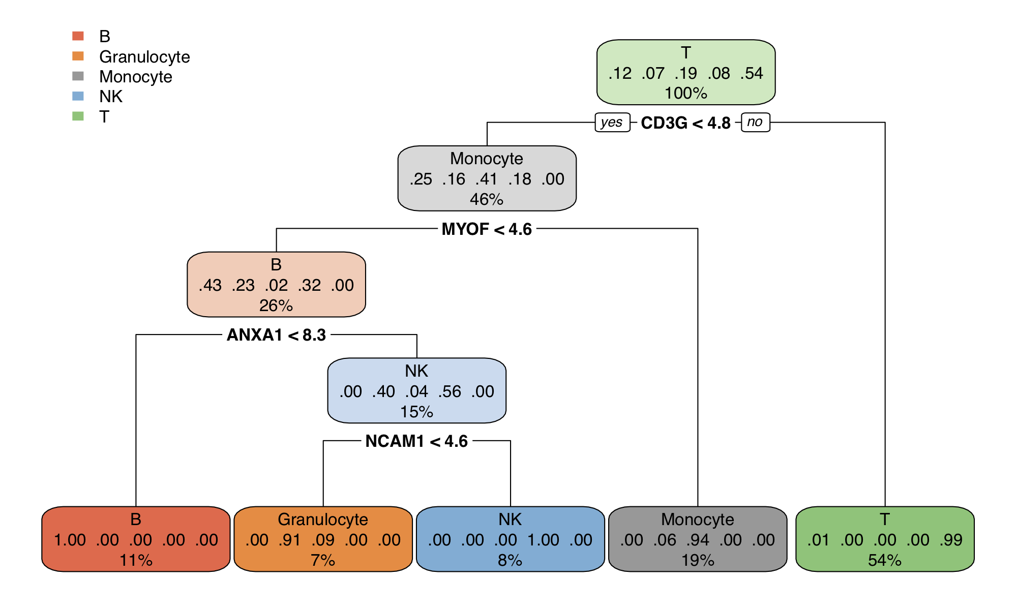
Figure 14. Classification tree for the rieckmann2017-immprot dataset. To reproduce similar figures, go to the Biomarker module, and set the Predicted target: cell.type from the input panel. Note that the classification tree is stochastically built up with some of the top features shown in Figure 10; Therefore, users can get a slightly different survival tree every time.

Volcano plots of methods

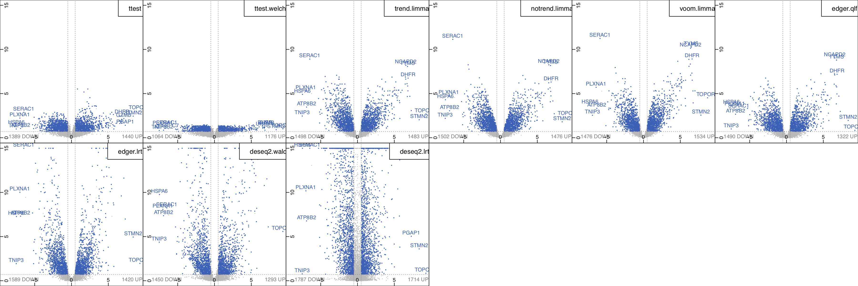
Figure 15. Volcano plots corresponding to eight different statistical methods comparing time-dependent expression of T cell activation at 48h vs. 12h. To regenerate the figure, select and load geiger2016-arginine dataset. Go to the Volcano (methods) panel under the Expression module, and set the Contrast: act48h_vs_act12h.